Tutorial
Introduction
This tutorial will guide you through the basic usage of the MMSBM library, showing how to work with nodes, metadata, and the bipartite network structure.
The nodes_layer Class
The nodes_layer class represents one type of nodes that forms the bipartite network. It can represent people, researchers, papers, metabolites, movies… That depends on your dataset.
The best way to initialize a nodes_layer is from a pandas DataFrame:
import pandas as pd
import numpy as np
from numba import jit
import sys, os
import BiMMSBM as sbm
from BiMMSBM.functions.utils import save_MMSBM_parameters,add_codes,load_EM_parameters

# Dataframe to use
df_politicians = pd.DataFrame({
    "legislator": ["Pedro", "Santiago", "Alberto", "Yolanda"],
    "Party": ["PSOE", "VOX", "PP", "Sumar"],
    "Movies_preferences": ["Action|Drama", "Belic", "Belic|Comedy", "Comedy|Drama"]
})

# Number of groups
K = 9
# You have to tell in which the name of the nodes will be as the second parameter
politicians = sbm.nodes_layer(K, "legislator", df_politicians)
Once the object is initialized, you can access the dataframe from the df attribute, but now it will contain a new column with an integer id that the library will use in the future. The name of the column is the same as the column of the names, but finished in _id.
display(politicians.df)
legislator |
Party |
Movies_preferences |
legislator_id |
|---|---|---|---|
Pedro |
PSOE |
Action|Drama |
1 |
Santiago |
VOX |
Belic |
2 |
Alberto |
PP |
Belic|Comedy |
0 |
Yolanda |
Sumar |
Comedy|Drama |
3 |
The assignment of the ids with the names of the nodes is in the dict_codes attribute and the inverse in the dict_decodes attribute. This ids represents the array position that corresponds to each node for the theta and omega matrices.
You can modify whenever you want the number of groups from the K attribute:
print(f"Number of groups of politicians: {politicians.K}")
politicians.K = 2
print(f"Number of groups of politicians: {politicians.K}")
Number of groups of politicians: 9
Number of groups of politicians: 2
Adding Metadata
When in your dataframe you have extra information about the nodes, you have to tell which columns are metadata and which type of metadata. There are two types of metadata:
Exclusive metadata: These are metadata where each node can only have assigned one attribute. For example the age of a person. A person only has one age, not more than one.
Inclusive metadata: These are metadata where each node can have assigned more than one attribute. For example the genre of a movie, one movie can belong to different genres at the same time.
Exclusive Metadata
Once the nodes_layer is initialized, you can add the metadata using the add_exclusive_metadata method that will return an exclusive_metadata class:
# Importance of the metadata
lambda_party = 100
parties = politicians.add_exclusive_metadata(lambda_party, "Party")
Also, this object will be stored inside the nodes_layer object in the meta_exclusives attribute that is a dictionary whose keys are the column names of the metadata and the value the object.
The value of lambda_party is how important the metadata will be while the inference procedure is running and it can be accessed from the lambda_val attribute:
print(f"Importance of political parties: {parties.lambda_val}")
parties.lambda_val = 2.3
print(f"Importance of political parties: {parties.lambda_val}")
Importance of political parties: 100
Importance of political parties: 2.3
When the metadata has been added to the nodes_layer object, its dataframe will add a new column with the ids of the metadata with the same column name but finished in _id.
display(politicians.df)
legislator |
Party |
Movies_preferences |
legislator_id |
Party_id |
|---|---|---|---|---|
Pedro |
PSOE |
Action|Drama |
1 |
1 |
Santiago |
VOX |
Belic |
2 |
3 |
Alberto |
PP |
Belic|Comedy |
0 |
0 |
Yolanda |
Sumar |
Comedy|Drama |
3 |
2 |
Similarly to the nodes_layer, you can access the metadata ids through the dict_codes attribute.
print(parties.dict_codes)
{'PSOE': 1, 'VOX': 3, 'PP': 0, 'Sumar': 2}
Inclusive Metadata
Once the nodes_layer is initialized, you can add the metadata using the add_inclusive_metadata method that will return an inclusive_metadata class:
# Importance of the metadata
lambda_movies = 0.3
# Number of groups of genres
Tau_movies = 6
movies = politicians.add_inclusive_metadata(lambda_movies, "Movies_preferences", Tau_movies)
Also, this object will be stored inside the nodes_layer object in the meta_inclusives attribute that is a dictionary whose keys are the column names of the metadata and the value the object.
The value of lambda_movies is how important the metadata will be while the inference procedure is running and it can be accessed from the lambda_val attribute:
print(f"Importance of politicians movies preferences: {movies.lambda_val}")
movies.lambda_val = 20
print(f"Importance of politicians movies preferences: {movies.lambda_val}")
Importance of politicians movies preferences: 0.3
Importance of politicians movies preferences: 20
The value of Tau_movies is the number of groups which the metadata will be grouped in the inference and it can be accessed from the Tau attribute:
print(f"Number of groups of politicians: {movies.Tau}")
movies.Tau = 3
print(f"Number of groups of politicians: {movies.Tau}")
Number of groups of politicians: 6
Number of groups of politicians: 3
When the metadata has been added to the nodes_layer object, its dataframe will add a new column with the ids of the metadata with the same column name but finished in _id.
display(politicians.df)
legislator |
Party |
Movies_preferences |
legislator_id |
Party_id |
Movies_preferences_id |
|---|---|---|---|---|---|
Pedro |
PSOE |
Action|Drama |
1 |
1 |
2|3 |
Santiago |
VOX |
Belic |
2 |
3 |
0 |
Alberto |
PP |
Belic|Comedy |
0 |
0 |
0|1 |
Yolanda |
Sumar |
Comedy|Drama |
3 |
2 |
1|3 |
Similarly to the nodes_layer, you can access the metadata ids through the dict_codes attribute.
Accessing Metadata Objects by Name
You can access the metadata_layer objects without using the meta_inclusive and meta_exclusives dictionaries:
politicians[str(movies)] == movies
politicians[str(parties)] == parties
BiNet Class
- The
BiNetclass contains the information about a bipartite network. It contains information about: Each of the layers that forms the bipartite network
The observed links.
BiNet Class Without Nodes Metadata
- To declare a
BiNetobject you need, at least, a dataframe with three columns: One with the source node
One with the target node
The label of the link
links_df = pd.DataFrame({
    "source": [0,0,0,1,1,1,2,2,2],
    "target": ["A","B","C","A","B","C","A","B","C"],
    "labels": ["positive","negative","positive","positive","negative","positive","negative","negative","positive"]
})
BiNet = sbm.BiNet(links_df, "labels", nodes_a_name="source", Ka=1, nodes_b_name="target", Kb=2)
Notice that you need to specify which columns represent nodes and which is the column of the labels. Also, because the class only distinguishes undirected networks, the columns assignments of nodes_a and nodes_b are irrelevant. Only the indexing of the matrices of the MMSBM parameters will be affected.
Once the object is initialized, you can access the dataframe from the df attribute, but now it will contain three new columns, one for each node type and another for the labels, with an integer id that the library will use in the future. The name of the column is the same as the column of the names, but finished in _id.
display(BiNet.df)
source |
target |
labels |
labels_id |
source_id |
target_id |
|---|---|---|---|---|---|
0 |
A |
positive |
1 |
0 |
0 |
0 |
B |
negative |
0 |
0 |
1 |
0 |
C |
positive |
1 |
0 |
2 |
1 |
A |
positive |
1 |
1 |
0 |
1 |
B |
negative |
0 |
1 |
1 |
1 |
C |
positive |
1 |
1 |
2 |
2 |
A |
negative |
0 |
2 |
0 |
2 |
B |
negative |
0 |
2 |
1 |
2 |
C |
positive |
1 |
2 |
2 |
Accessing the nodes_layer Objects
Two attributes that contain the information of the nodes are the nodes_a and nodes_b attributes, which are nodes_layer objects.
print(BiNet.nodes_a, type(BiNet.nodes_a))
print(BiNet.nodes_b, type(BiNet.nodes_b))
source <class 'BiMMSBM.nodes_layer'>
target <class 'BiMMSBM.nodes_layer'>
An easier way to access these objects is by using the name of the layer:
print(BiNet["source"] == BiNet.nodes_a)
print(BiNet["target"] == BiNet.nodes_b)
True
True
As before, you can access a dataframe with the df method. Also, it will contain an extra column with the ids.
display(BiNet["source"].df)
source |
source_id |
|---|---|
0 |
0 |
1 |
1 |
2 |
2 |
target |
target_id |
|---|---|
A |
0 |
B |
1 |
C |
2 |
Using nodes_layer Objects to Initialize a BiNet Object
The previous example only has a link list with labels. Sometimes you want to infer using nodes’ metadata. The best way to do that is by using nodes_layer objects.
First, let’s create the nodes_layer objects:
# Dataframe to use
df_politicians = pd.DataFrame({
    "legislator": ["Pedro", "Santiago", "Alberto", "Yolanda"],
    "Party": ["PSOE", "VOX", "PP", "Sumar"],
    "Movies_preferences": ["Action|Drama", "Belic", "Belic|Comedy", "Comedy|Drama"]
})
# Number of groups
K = 2
politicians = sbm.nodes_layer(K, "legislator", df_politicians)
politicians.add_exclusive_metadata(1, "Party")
politicians.add_inclusive_metadata(1, "Movies_preferences", 1)

# Dataframe to use
df_bills = pd.DataFrame({
    "bill": ["A", "B", "C", "D"],
    "Year": [2020, 2020, 2021, 2022]
})
K = 2
bills = sbm.nodes_layer(K, "bill", df_bills)
Now we can create the BiNet object, but with the difference that instead of specifying the name of the nodes layer, you have to use as a parameter the nodes_layer object using the nodes_a and nodes_b parameters.
# Dataframe to use
df_votes = pd.DataFrame({
    "legislator": ["Pedro","Pedro","Pedro","Santiago","Santiago","Santiago",
                   "Alberto", "Alberto", "Alberto", "Yolanda", "Yolanda", "Yolanda"],
    "bill": ["A", "B", "D",  "A","C", "D",
             "A", "B", "C",  "B","C", "D",],
    "votes": ["Yes","No","No",  "No","Yes","Yes",
              "No","No","Yes",  "Yes","No","No"]
})
# Creating the BiNet object
votes = sbm.BiNet(df_votes, "votes", nodes_a=bills, nodes_b=politicians)
Notice that you do not need to specify the number of the groups of each nodes_layer because it is contained in the corresponding nodes_layer.
Important
The name of the columns of the layer in both DataFrames (from the nodes_layer object and for the BiNet object) must coincide. Else, a KeyError will arise.
It is not mandatory to use two nodes_layer to create the BiNet object when you need metadata from only one of the layers. Remember to specify the number of groups.
# Example using only one nodes_layer object
votes = sbm.BiNet(df_votes, "votes", nodes_a_name="bill", Ka=2, nodes_b=politicians)
If you display the dataframe of the BiNet and the nodes_layer objects, the nodes ids from both layers will coincide.
display(votes.df[["legislator","legislator_id","bill","bill_id"]])
display(votes["legislator"].df[["legislator","legislator_id"]])
display(votes["bill"].df[["bill","bill_id"]])
legislator |
legislator_id |
bill |
bill_id |
|---|---|---|---|
Pedro |
1 |
A |
0 |
Pedro |
1 |
B |
1 |
Pedro |
1 |
D |
3 |
Santiago |
2 |
A |
0 |
Santiago |
2 |
C |
2 |
Santiago |
2 |
D |
3 |
Alberto |
0 |
A |
0 |
Alberto |
0 |
B |
1 |
Alberto |
0 |
C |
2 |
Yolanda |
3 |
B |
1 |
Yolanda |
3 |
C |
2 |
Yolanda |
3 |
D |
3 |
legislator |
legislator_id |
|---|---|
Pedro |
1 |
Santiago |
2 |
Alberto |
0 |
Yolanda |
3 |
bill |
bill_id |
|---|---|
A |
0 |
B |
1 |
D |
3 |
C |
2 |
The Expectation Maximization (EM) algorithm
To start to infer the parameters of the MMSBM, you have to initialize the parameters. It can be easily done with the init_EM method.
votes.init_EM()
Once the EM has been initialized, the parameters will be stored in attributes. For the membership parameters, each nodes_layer will have a theta attribute that is a matrix.
votes["legislator"].theta
array([[0.39067672, 0.60932328],
       [0.51318295, 0.48681705],
       [0.23656348, 0.76343652],
       [0.8699203 , 0.1300797 ]])
votes["bill"].theta
array([[0.33855864, 0.66144136],
       [0.10264972, 0.89735028],
       [0.33213194, 0.66786806],
       [0.43570408, 0.56429592]])
The first index corresponds to the id of the node, the second correspond to the group number.
For the BiNet object, the probabilities matrix and the expectation parameters will be stored in the pkl and omega attributes respectivly.
votes.pkl
array([[[0.73640347, 0.26359653],
        [0.66204141, 0.33795859]],

       [[0.61438835, 0.38561165],
        [0.7342769 , 0.2657231 ]]])
The first and second index corresponds to the groups from nodes_a and nodes_b respectively. The third correspond to the label id.
votes.omega
array([[[[0.14143346, 0.19831325],
        [0.23053494, 0.42971834]],

        [[0.14403937, 0.17518567],
        [0.41166991, 0.26910505]],

        [[0.08461626, 0.24549825],
        [0.13792355, 0.53196193]],

        [[0.        , 0.        ],
        [0.        , 0.        ]]],


      [[[0.04293584, 0.06020319],
        [0.31314921, 0.58371176]],

       [[0.05742163, 0.04897093],
        [0.4188002 , 0.47480724]],

       [[0.        , 0.        ],
        [0.        , 0.        ]],

       [[0.06536891, 0.01253214],
        [0.83596087, 0.08613808]]],


     [[[0.10985576, 0.21967309],
        [0.32315681, 0.34731435]],

      [[0.        , 0.        ],
        [0.        , 0.        ]],

      [[0.0683947 , 0.28299025],
        [0.20119303, 0.44742201]],

      [[0.32134512, 0.04319874],
        [0.53911187, 0.09634426]]],


     [[[0.        , 0.        ],
        [0.        , 0.        ]],

      [[0.24047583, 0.2050852 ],
        [0.2598447 , 0.29459428]],

      [[0.08892354, 0.36793049],
        [0.16847772, 0.37466824]],

      [[0.41526893, 0.05582501],
        [0.44871632, 0.08018974]]]])
The first and second index corresponds to the nodes id from nodes_a and nodes_b respectively. The second and third index corresponds to the groups from nodes_a and nodes_b respectively.
Running the EM Algorithm and Checking Convergence
To run the EM algorithm, you have to use the EM_step method. It will make an iteration of the algorithm by default. You can specify the number of iterations with the N_steps parameter. To check the convergence, you can use the converges method.
N_itt = 100
N_check = 5  # Number of iterations to measure the convergence

for itt in range(N_itt//N_check):
    votes.EM_step(N_check)
    converges = votes.converges()
    print(f"Iteration {itt*N_check}: {converges}")
    if converges:
        break
Iteration 0: False
Iteration 5: False
Iteration 10: False
Iteration 15: False
Iteration 20: True
Using Training Sets and Test Sets
You can select a training set instead of using all the links to infer the parameters. You can do that using the training parameter when you initialize the EM algorithm.
This parameter can be a list of the links ids that you want to use as a training set, or another dataframe with more links. If not specified, all the links will be used.
from sklearn.model_selection import train_test_split

# Defining the training and test sets
df_train, df_test = train_test_split(votes.df, test_size=0.2)

# Initializing the EM algorithm with the training set
votes.init_EM(training=df_train)

# Running the EM algorithm
N_itt = 100
N_check = 5  # Number of iterations to measure the convergence
for itt in range(N_itt//N_check):
    votes.EM_step(N_check)
    converges = votes.converges()
    print(f"Iteration {itt*N_check}: converges? {converges}")
    if converges:
        break
Iteration 0: converges? False
Iteration 5: converges? False
Iteration 10: converges? False
Iteration 15: converges? False
Iteration 20: converges? False
Iteration 25: converges? False
Iteration 30: converges? False
Iteration 35: converges? False
Iteration 40: converges? False
Iteration 45: converges? True
Checking the Accuracy and Getting Predictions
Once the EM algorithm has converged, you can get the predictions using the get_predicted_labels method. You can specify which links you want to infer its labels with the links parameter. If no links are specified, it will use the links used for training the model.
votes.get_predicted_labels()
votes.get_predicted_labels(links=df_test)
Checking the Accuracy
You can check the accuracy of the predictions using the get_accuracy method. By default, it will compute the accuracy of the training set. You can specify the test set with the links parameter, by using a list of the links ids or another dataframe with other links.
# Accuracy of the training set
print(f"Accuracy of the training set: {votes.get_accuracy()}")
print(f"Accuracy of the test set: {votes.get_accuracy(links=df_test)}")
Accuracy of the training set: 0.8888888888888888
Accuracy of the test set: 0.0
Saving and Loading the Parameters
For long runs or for using the parameters later, you can save the parameters. It is very important to notice that it is also important to save the ids of the nodes and labels, and some information of the nodes_layer and BiNet objects before initializing the EM algorithm. To save the parameters you can use the save_nodes_layer and save_BiNet methods.
The save_nodes_layer Method
This method is useful when you only want to save the information of a nodes_layer object. One example can be when you want to do a 5-fold cross-validation, instead of saving the nodes information for each fold, you can save it once and load it later once for all the folds.
The name of the JSON will be layer_{nodes_layer.name}_data.json.
Saving the Parameters with save_MMSBM_parameters Function
To save the parameters of the EM procedure, you can use the save_MMSBM_parameters function:
from MMSBM_library.functions.utils import save_MMSBM_parameters

from sklearn.model_selection import train_test_split

try:
    os.mkdir("tutorial_saves")
    os.mkdir("tutorial_saves/example_BiNet")
    os.mkdir("tutorial_saves/example_parameters")
except:
    pass

# Defining the training and test sets
df_train, df_test = train_test_split(votes.df, test_size=0.2)

votes.save_BiNet("./tutorial_saves/example_BiNet/")

# Initializing the EM algorithm with the training set
votes.init_EM(training=df_train)

# Running the EM algorithm
N_itt = 100
N_check = 5  # Number of iterations to measure the convergence
for itt in range(N_itt//N_check):
    votes.EM_step(N_check)
    converges = votes.converges()
    print(f"Iteration {itt*N_check}: converges? {converges}")
    if converges:
        save_MMSBM_parameters(votes, "./tutorial_saves/example_parameters")
        break
- Now different .npy files have been created inside example_parameters folder:
theta_a.npy and theta_b.npy contain the parameters of the nodes_layer objects that form the BiNet object.
pkl.npy contains the membership probabilities.
For each exclusive metadata it will generate: - qka_{meta_name}.npy with the membership probability for each metadata.
For each inclusive metadata it will generate: - q_k_tau_{meta_name}.npy with the membership probability for each metadata. - zeta_{meta_name}.npy with the membership factors for each metadata.
The load_BiNet_from_json and the init_EM_from_directory methods
Also, you can load your saved BiNet class using the load_BiNet_from_json class method:
loaded_votes = sbm.BiNet.load_BiNet_from_json("./tutorial_saves/example_BiNet/BiNet_data.json",
                                              links=df_votes, links_label="votes",
                                              nodes_a=bills, nodes_b=politicians)
If you want to load the parameters obtained from an EM procedure to continue the procedure or to analyze the parameters, you have to use the init_EM_from_directory method.
loaded_votes.init_EM_from_directory(dir="./tutorial_saves/example_parameters", training=df_train)
From here you can continue the EM procedure using the EM_step method:
loaded_votes.df
loaded_votes.EM_step(10)
Or analyze the parameters and/or links and/or accuracies:
loaded_votes.df
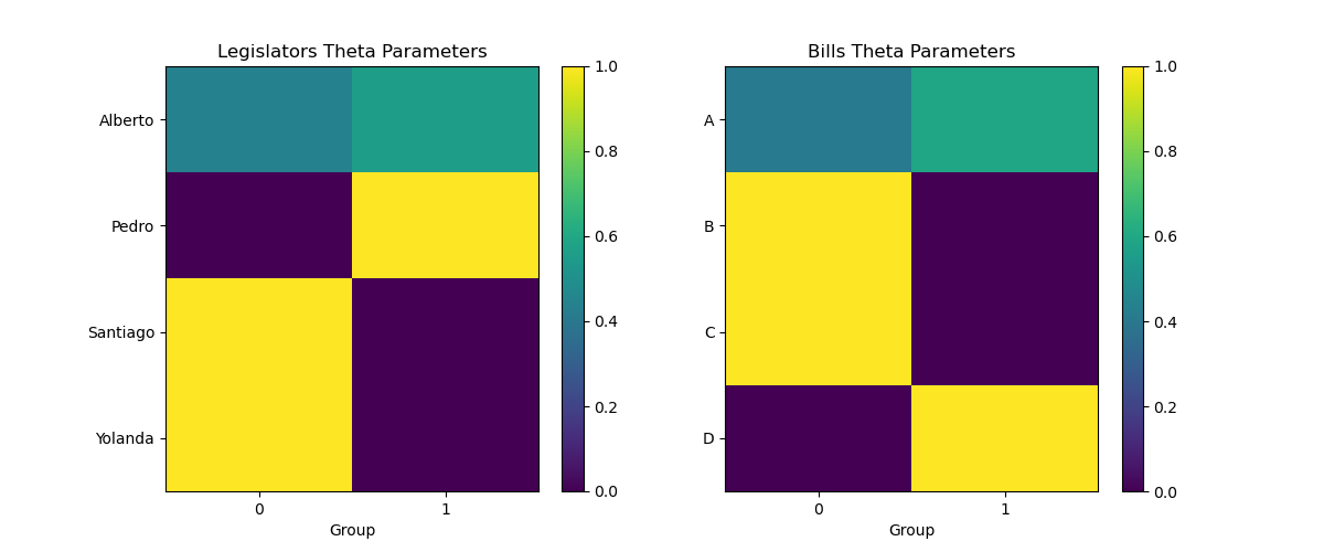
Plotting the Membership Matrices
You can visualize the membership matrices of the politicians and the votes using matplotlib:
import matplotlib.pyplot as plt

fig, (ax1, ax2) = plt.subplots(1, 2, figsize=(12, 5))
# Plot theta parameters for both nodes as heatmaps
im1 = ax1.imshow(loaded_votes.nodes_a.theta, cmap='viridis', aspect='auto')
im2 = ax2.imshow(loaded_votes.nodes_b.theta, cmap='viridis', aspect='auto')

# Add colorbars
plt.colorbar(im1, ax=ax1)
plt.colorbar(im2, ax=ax2)

# Set titles
ax1.set_title('Legislators Theta Parameters')
ax2.set_title('Bills Theta Parameters')

# Label axes
ax1.set_xlabel('Group')
ax2.set_xlabel('Group')

# Set y-tick labels to node IDs
ax1.set_yticks(range(len(politicians)))
ax1.set_yticklabels([politicians.dict_decodes[i] for i in range(len(politicians))])
ax2.set_yticks(range(len(bills)))
ax2.set_yticklabels([bills.dict_decodes[i] for i in range(len(bills))])

ax1.set_xticks(range(politicians.K))
ax2.set_xticks(range(bills.K))